Ten Easy Ways to Estimate How Many Participants You Need

IN THIS CHAPTER

Quickly estimating sample size for several basic statistical tests

Adjusting for different levels of power and α

Adjusting for unequal group sizes and for attrition during the study

Sample-size calculations (also called power calculations) tend to frighten researchers and send them running to the nearest statistician. But if you you need a ballpark idea of how many participants are needed for a new research project, you can use these ten quick and dirty rules of thumb.

Before you begin, take a look at Chapter 3 — especially the sections on hypothesis testing and the power of a test. That way, you’ll refresh your memory about what power and sample-size calculations are all about. For your study, you will need to select the effect size of importance that you want to detect. An effect size could be the difference of at least 10 mmHg in mean systolic blood-pressure lowering between groups on two different hypertension drugs, or it could be having the degree of correlation between two laboratory values of at least 0.7. Once you select your effect size and compatible statistical test, look in this chapter for the rule for the statistical test you selected to calculate the sample size.

The first six sections tell you how many participants you need to provide complete data for you to analyze in order to have an 80 percent chance of getting a p value that’s less than 0.05 when you run the test if a true difference of your effect size does indeed exist. In other words, we are setting the parameters 80 percent power at α = 0.05, because they are widely used in biological research. The remaining four sections tell you how to modify your estimate for other power or α values, and how to adjust your estimate for unequal group size and dropouts from the study.

Comparing Means between Two Groups

• Applies to: Unpaired Student t test, Mann-Whitney U test, and Wilcoxon Sum-of-Ranks test.
• Effect size (E): The difference between the means of two groups divided by the standard deviation (SD) of the values within a group.
• Rule: You need participants in each group, or participants altogether.

For example, say you’re comparing two hypertension drugs — Drug A and Drug B — on lowering systolic blood pressure (SBP). You might set the effect size of 10 mmHg. You also know from prior studies that the SD of the SBP change is known to be 20 mmHg. Then the equation is , or 0.5, and you need , or 64 participants in each group (128 total).

Comparing Means among Three, Four, or Five Groups

• Applies to: One-way Analysis of Variance (ANOVA) or Kruskal-Wallis test.
• Effect size (E): The difference between the largest and smallest means among the groups divided by the within-group SD.
• Rule: You need participants in each group.

Continuing the example from the preceding section, if you’re comparing three hypertension drugs — Drug A, Drug B, and Drug C — and if any mean difference of 10 mmHg in SBP between any pair of drug groups is important, then E is still , or 0.5, but you now need , or 80 participants in each group (240 total).

Comparing Paired Values

• Applies to: Paired Student t test or Wilcoxon Signed-Ranks test.
• Effect size (E): The average of the paired differences divided by the SD of the paired differences.
• Rule: You need participants (pairs of values).

Imagine that you’re studying test scores in struggling students before and after tutoring. You determine a six-point improvement in grade points is the effect size of importance, and the SD of the changes is ten points. Then , or 0.6, and you need , or about 22 students, each of whom provides a before score and an after score.

Comparing Proportions between Two Groups

• Applies to: Chi-square test of association or Fisher Exact test.
• Effect size (D): The difference between the two proportions ( and ) that you’re comparing. You also have to calculate the average of the two proportions: .
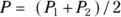• Rule: You need 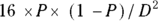participants in each group.

For example, if a disease has a 60 percent mortality rate, but you think your drug can cut this rate in half to 30 percent, then 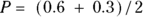, or 0.45, and , or 0.3. You need , or 44 participants in each group (88 total).

Testing for a Significant Correlation

• Applies to: Pearson correlation test. It is also a good approximation for the non-parametric Spearman correlation test.
• Effect size: The correlation coefficient (r) you want to be able to detect.
• Rule: You need participants (pairs of values).

Imagine that you’re studying the association between weight and blood pressure, and you want the correlation test to come out statistically significant if these two variables have a true correlation coefficient of at least 0.2. Then you need to study , or 200 participants.

Comparing Survival between Two Groups

• Applies to: Log-rank test or Cox proportional-hazard regression.
• Effect size: The hazard ratio (HR) you want to be able to detect.
• Rule: The required total number of observed deaths/events .

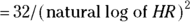Here’s how the formula works out for several values of HR greater than 1:

Your enrollment must be large enough and your follow-up must be long enough to ensure that the required number of events take place during the observation period. This may be difficult to estimate beforehand as it involves considering recruitment rates, censoring rates, the shape of the survival curve, and other factors difficult to forecast. Some research protocols provide only a tentative estimate of the expected enrollment for planning, budgeting, and ethical purposes. Many state that enrollment and/or follow-up will continue until the required number of events has been observed. Even with ambiguity, it is important to follow conventions described in this book when designing to avoid criticism for departing from good general principles.

Scaling from 80 Percent to Some Other Power

Here’s how you take a sample-size estimate that provides 80 percent power from one of the preceding rules and scale it up or down to provide some other power:

• For 50 percent power: Use only half as many participants — multiply the estimate by 0.5.
• For 90 percent power: Increase the sample size by 33 percent — multiply the estimate by 1.33.
• For 95 percent power: Increase the sample size by 66 percent — multiply the estimate by 1.66.

For example, if you know from doing a prior sample size calculation that a study with 70 participants provides 80 percent power to test its primary objective, then a study that has , or 93 participants will have about 90 percent power to test the same objective. The reason to consider power of levels other than 80 percent is because of limited sample. If you know that 70 participants provides 80 percent power, but you will only have access to 40, you can estimate maximum power you are able to achieve.

Scaling from 0.05 to Some Other Alpha Level

Here’s how you take a sample-size estimate that was based on testing at the α = 0.05 level, and scale it up or down to correspond to testing at some other α level:

• For α = 0.10: Decrease the sample size by 20 percent — multiply the estimate by 0.8.
• For α = 0.025: Increase the sample size by 20 percent — multiply the estimate by 1.2.
• For α = 0.01: Increase the sample size by 50 percent — multiply the estimate by 1.5.

For example, imagine that you’ve calculated you need a sample size of 100 participants using α = 0.05 as your criterion for significance. Then your boss says you have to apply a two-fold Bonferroni correction (see Chapter 11) and use α = 0.025 as your criterion instead. You need to increase your sample size to 100 x 1.2, or 120 participants, to have the same power at the new α level.

Adjusting for Unequal Group Sizes

When comparing means or proportions between two groups, you usually get the best power for a given sample size — meaning it’s more efficient — if both groups are the same size. If you don’t mind having unbalanced groups, you will need more participants overall in order to preserve statistical power. Here’s how to adjust the size of the two groups to keep the same statistical power:

• If you want one group twice as large as the other: Increase one group by 50 percent, and reduce the other group by 25 percent. This increases the total sample size by about 13 percent.
• If you want one group three times as large as the other: Reduce one group by a third, and double the size of the other group. This increases the total sample size by about 33 percent.
• If you want one group four times as large as the other: Reduce one group by 38 percent and increase the other group by 250 percent. This increases the total sample size by about 56 percent.

Suppose that you’re comparing two equal-sized groups, Drug A and Drug B. You’ve calculated that you need two groups of 32, for a total of 64 participants. Now, you decide to randomize group assignment using a 2:1 ratio for A:B. To keep the same power, you’ll need , or 48 for Drug A, an increase of 50 percent. For B, you’ll want , or 24, a decrease of 25 percent, for an overall new total 72 participants in the study.

Allowing for Attrition

Sample size estimates apply to the number of participants who give you complete, analyzable data. In reality, you have to increase this estimate to account for those who will drop out of the study, or provide incomplete data for other reasons (called attrition). Here’s how to scale up your sample size estimate to develop an enrollment target that compensates for attrition, remembering longer duration studies may have higher attrition:

Enrollment = Number Providing Complete Data × 100/(100 – %Attrition)

Here are the enrollment scale-ups for several attrition rates:

If your sample size estimate says you need a total of 60 participants with complete data, and you expect a 25 percent attrition rate, you need to enroll , or 80 participants. That way, you’ll have complete data on 60 participants after a quarter of the original 80 are removed from analysis.